New computer vision system designed to analyse cells in microscopy videos

Researchers have developed a system based on computer vision techniques that allows automatic analysis of biomedical videos captured by microscopy in order to characterize and describe the behavior of the cells that appear in the images.

source https://www.sciencedaily.com/releases/2022/02/220211102608.htm

Novel wearable armband helps users of prosthetic hands to ‘get a grip’

A new study could be a game changer for users of prosthetic hands who have long awaited advances in dexterity. Researchers examined if people could precisely control the grip forces applied to two different objects grasped simultaneously with a dexterous artificial hand. They designed a multichannel wearable soft robotic armband to convey artificial sensations of touch to the robotic hand users. Subjects were able to successfully grasp and transport two objects simultaneously with the dexterous artificial hand without breaking or dropping them, even when their vision of both objects was obstructed. The study is the first to show the feasibility of this complex simultaneous control task while integrating multiple channels of haptic/touch sensation feedback noninvasively.

source https://www.sciencedaily.com/releases/2022/02/220211080635.htm

Comments, docstrings, and type hints in Python code

Tweet Tweet Share Share

The source code of a program should be readable to human. Making it run correctly is only half of its purpose. Without a properly commenting code, it would be difficult for one, including the future you, to understand the rationale and intent behind the code. It would also make the code impossible to maintain. In Python, there are multiple ways to add descriptions to the code to make it more readable or make the intent more explicit. In the following, we will see how we should properly use comments, docstrings, and type hints to make our code easier to understand. After finishing this tutorial, you will know

• What is the proper way of using comments in Python
• How string literal or docstring can replace comments in some cases
• What is type hints in Python and how it can help us understand the code better

Let’s get started.

Comments, docstrings, and type hints in Python code. Photo by Rhythm Goyal. Some rights reserved

Overview

This tutorial is in 3 parts, they are

• Adding comments to Python code
• Using docstrings
• Using type hints in Python code

Adding comments to Python code

Almost all programming languages have dedicated syntax for comments. Comments are to be ignored by compilers or interpreters and hence they have no effect to the programming flow or logic. But with comments, we are easier to read the code.

In languages like C++, we can add “inline comments” with a leading double slash (//) or add comment blocks enclosed by /* and */. However, in Python we only have the “inline” version and they are introduced by the leading hash character (#).

It is quite easy to write comments to explain every line of code but usually that is a waste. When people read the source code, quite often comments are easier to catch attention and hence putting too much comments would distract the reading. For example, the following is unnecessary and distracting:

import datetime
 

 
timestamp = datetime.datetime.now()  # Get the current date and time
 
x = 0    # initialize x to zero

Comments like these is merely repeating what the code does. Unless the code is obscured, these comments added no value to the code. The example below might be a marginal case, in which the name “ppf” (percentage point function) is less well-known than the term “CDF” (cumulative distribution function):

import scipy.stats
 

 
z_alpha = scipy.stats.norm.ppf(0.975)  # Call the inverse CDF of standard normal

Good comments should be telling why we are doing something. Let’s look at the following example:

def adadelta(objective, derivative, bounds, n_iter, rho, ep=1e-3):
 
    # generate an initial point
 
    solution = bounds[:, 0] + rand(len(bounds)) * (bounds[:, 1] - bounds[:, 0])
 
    # lists to hold the average square gradients for each variable and
 
    # average parameter updates
 
    sq_grad_avg = [0.0 for _ in range(bounds.shape[0])]
 
    sq_para_avg = [0.0 for _ in range(bounds.shape[0])]
 
    # run the gradient descent
 
    for it in range(n_iter):
 
        gradient = derivative(solution[0], solution[1])
 
        # update the moving average of the squared partial derivatives
 
        for i in range(gradient.shape[0]):
 
            sg = gradient[i]**2.0
 
            sq_grad_avg[i] = (sq_grad_avg[i] * rho) + (sg * (1.0-rho))
 
        # build a solution one variable at a time
 
        new_solution = list()
 
        for i in range(solution.shape[0]):
 
            # calculate the step size for this variable
 
            alpha = (ep + sqrt(sq_para_avg[i])) / (ep + sqrt(sq_grad_avg[i]))
 
            # calculate the change and update the moving average of the squared change
 
            change = alpha * gradient[i]
 
            sq_para_avg[i] = (sq_para_avg[i] * rho) + (change**2.0 * (1.0-rho))
 
            # calculate the new position in this variable and store as new solution
 
            value = solution[i] - change
 
            new_solution.append(value)
 
        # evaluate candidate point
 
        solution = asarray(new_solution)
 
        solution_eval = objective(solution[0], solution[1])
 
        # report progress
 
        print('>%d f(%s) = %.5f' % (it, solution, solution_eval))
 
    return [solution, solution_eval]

The function above is implementing AdaDelta algorithm. At the first line, when we assign something to the variable solution, we do not write comments like “a random interpolation between bounds[:,0] and bounds[:,1]” because that is just repeating the code literally. We say the intent of this line is to “generate an initial point”. Similarly for the other comments in the function, we mark one of the for loop as the gradient descent algorithm rather than just saying iterate for certain times.

One important issue we want to remember when writing the comment or modifying code is to make sure the comment accurately describe the code. If they are contradicting, it would be confusing to the readers. If we should not put the comment on the first line of the above example to “set initial solution to the lowerbound” while the code obviously is randomizing the initial solution, or vice versa. If this is what you intented to do, you should update the comment and the code at the same time.

An exception would be the “to-do” comments. From time to time, when we have an idea on how to improve the code but not yet changed it, we may put a to-do comments on the code. We can also use it to mark incomplete implementations. For example,

# TODO replace Keras code below with Tensorflow
 
from keras.models import Sequential
 
from keras.layers import Conv2D
 

 
model = Sequential()
 
model.add(Conv2D(1, (3,3), strides=(2, 2), input_shape=(8, 8, 1)))
 
model.summary()
 
...

This is a common practice and many IDE will highlight the comment block differently when the keyword TODO is found. However, it suppposed to be temporary and we should not abuse it as an issue tracking system.

In summary, some common “best practice” on commenting code as listed as follows:

• Comments should not restate the code, but to explain it
• Comments should not cause confusion, but to eliminate it
• Put comments on code that is not trivial to understand, for example, state the unidiomatic use of syntax, name the algorithm being used, or explain the intent or assumptions
• Comments should be concise and simple
• Keep a consistent style and use of language in commenting
• Always prefer to have a better written code that needs no additional comment

Using docstrings

In C++, we may write a large block of comments such as in the following:

TcpSocketBase::~TcpSocketBase (void)
 
{
 
  NS_LOG_FUNCTION (this);
 
  m_node = nullptr;
 
  if (m_endPoint != nullptr)
 
    {
 
      NS_ASSERT (m_tcp != nullptr);
 
      /*
 
       * Upon Bind, an Ipv4Endpoint is allocated and set to m_endPoint, and
 
       * DestroyCallback is set to TcpSocketBase::Destroy. If we called
 
       * m_tcp->DeAllocate, it will destroy its Ipv4EndpointDemux::DeAllocate,
 
       * which in turn destroys my m_endPoint, and in turn invokes
 
       * TcpSocketBase::Destroy to nullify m_node, m_endPoint, and m_tcp.
 
       */
 
      NS_ASSERT (m_endPoint != nullptr);
 
      m_tcp->DeAllocate (m_endPoint);
 
      NS_ASSERT (m_endPoint == nullptr);
 
    }
 
  if (m_endPoint6 != nullptr)
 
    {
 
      NS_ASSERT (m_tcp != nullptr);
 
      NS_ASSERT (m_endPoint6 != nullptr);
 
      m_tcp->DeAllocate (m_endPoint6);
 
      NS_ASSERT (m_endPoint6 == nullptr);
 
    }
 
  m_tcp = 0;
 
  CancelAllTimers ();
 
}

But in Python, we do not have the equivalent to the delimiters /* and */, but we can write multi-line comments like the following instead:

async def main(indir):
 
    # Scan dirs for files and populate a list
 
    filepaths = []
 
    for path, dirs, files in os.walk(indir):
 
        for basename in files:
 
            filepath = os.path.join(path, basename)
 
            filepaths.append(filepath)
 

 
    """Create the "process pool" of 4 and run asyncio.
 
    The processes will execute the worker function
 
    concurrently with each file path as parameter
 
    """
 
    loop = asyncio.get_running_loop()
 
    with concurrent.futures.ProcessPoolExecutor(max_workers=4) as executor:
 
        futures = [loop.run_in_executor(executor, func, f) for f in filepaths]
 
        for fut in asyncio.as_completed(futures):
 
            try:
 
                filepath = await fut
 
                print(filepath)
 
            except Exception as exc:
 
                print("failed one job")

This works because Python supports to declare a string literal spanning across multiple lines if it is delimited with triple quotation marks ("""). And a string literal in the code is merely a string declared with no impact. Therefore it is functionally no different to the comments.

One reason we want to use string literals is to comment out a large block of code. For example,

from sklearn.linear_model import LogisticRegression
 
from sklearn.datasets import make_classification
 
"""
 
X, y = make_classification(n_samples=5000, n_features=2, n_informative=2,
 
                           n_redundant=0, n_repeated=0, n_classes=2,
 
                           n_clusters_per_class=1,
 
                           weights=[0.01, 0.05, 0.94],
 
                           class_sep=0.8, random_state=0)
 
"""
 
import pickle
 
with open("dataset.pickle", "wb") as fp:
 
    X, y = pickle.load(fp)
 

 
clf = LogisticRegression(random_state=0).fit(X, y)
 
...

The above is a sample code that we may develop with experimenting on a machine learning problem. While we generated a dataset randomly at the beginning (the call to make_classification() above), we may want to switch to a different dataset and repeat the same process at a later time (e.g., the pickle part above). Rather than removing the block of code, we may simply comment those lines so we can store the code later. It is not in a good shape for the finalized code but convenient while we are developing our solution.

The string literal in Python as comment has a special purpose if it is at the first line under a function. The string literal in that case is called the “docstring” of the function. For example,

def square(x):
 
    """Just to compute the square of a value
 
    
 
    Args:
 
        x (int or float): A numerical value
 

 
    Returns:
 
        int or float: The square of x
 
    """
 
    return x * x

We can see the first line under the function is a literal string and it serve as the same purpose as comment. It makes the code more readable, but at the same time, we can retrieve it from the code:

print("Function name:", square.__name__)
 
print("Docstring:", square.__doc__)

Function name: square
 
Docstring: Just to compute the square of a value
 
    
 
    Args:
 
        x (int or float): A numerical value
 

 
    Returns:
 
        int or float: The square of x

Because of the special status of the docstring, there are several conventions on how to write a proper one.

In C++ we may use Doxygen to generate code documentation from comments and similarly we have Javadoc for Java code. The closest match in Python would be the tool “autodoc” from Sphinx or pdoc. Both will try to parse the docstring to generate documentations automatically.

There are no standard way of making docstrings but generally we expect they will explain the purpose of a function (or a class or module) as well as the arguments and the return values. One common style is like the one above, which is advocated by Google. A different style is from NumPy:

def square(x):
 
    """Just to compupte the square of a value
 
    
 
    Parameters
 
    ----------
 
    x : int or float
 
        A numerical value
 

 
    Returns
 
    -------
 
    int or float
 
        The square of `x`
 
    """
 
    return x * x

Tools such as autodoc can parse these docstring and generate the API documentation. But even if it is not the purpose, having a docstring describing the nature of the function, the data types of the function arguments and return values can surely make your code easier to read. This is particularly true since Python, unlike C++ or Java, is a duck-typing language which variables and function arguments are not declared with a particular type. We can make use of docstring to spell out the assumption of the data type so people are easier to follow or use your function.

Using type hints in Python code

Since Python 3.5, type hint syntax is allowed. As the name implies, its purpose is to hint for the type, and nothing else. Hence even it looks like to bring Python closer to Java, it does not mean to restrict the data to be stored in a variable. The example above can be rewritten with type hint:

def square(x: int) -> int:
 
    return x * x

In a function, the arguments can be followed by a : type syntax to spell out the intended types. The return value of a function is identified by the -> type syntax before the colon. In fact, type hint can be declared for variables too, e.g.,

def square(x: int) -> int:
 
    value: int = x * x
 
    return value

The benefit of type hint is two fold: We can use it to eliminate some comments if we need to describe explicitly the data type being used. We can also help static analyzers to understand our code better so they can help identifying potential issues in the code.

Sometimes the type can be complex and therefore Python provided the typing module in its standard library to help clean up the syntax. For example, we can use Union[int,float] to mean int type or float type, List[str] to mean a list that every element is a string, and use Any to mean anything. Like as follows:

from typing import Any, Union, List
 

 
def square(x: Union[int, float]) -> Union[int, float]:
 
    return x * x
 

 
def append(x: List[Any], y: Any) -> None:
 
    x.append(y)

However, it is important to remember that type hints are hints only. It does not impose any restriction to the code. Hence the following is confusing to the reader, but perfectly fine:

n: int = 3.5
 
n = "assign a string"

Using type hints may improve the readability of the code. However, the most important benefit of type hint is to allow static analyzer such as mypy to tell us whether our code has any potential bug. If you process the above lines of code with mypy, we will see the following error:

test.py:1: error: Incompatible types in assignment (expression has type "float", variable has type "int")
 
test.py:2: error: Incompatible types in assignment (expression has type "str", variable has type "int")
 
Found 2 errors in 1 file (checked 1 source file)

The use of static analyzers will be covered in another post.

To illustrate the use of comments, docstrings, and type hints, below is an example to define a generator function that samples a pandas DataFrame on fixed-width windows. It is useful for training a LSTM network, which a few consecutive time steps should be provided. In the function below, we start from a random row on the DataFrame and clip a few rows following it. As long as we can successfully get one full window, we take it as a sample. Once we collected enough samples to make a batch, the batch is dispatched.

You should see that it is clearer if we can provide type hints on the function arguments so we know, for example, data is supposed to be a pandas DataFrame. But we describe further that it is expected to carry a datetime index in the docstring. The describe the algorithm on how to exact a window of rows from the input data as well as the intention of the “if” block in the inner while-loop using comments. In this way, the code would be much easier to understand and much easier to maintain, or modified for other use.

from typing import List, Tuple, Generator
 
import pandas as pd
 
import numpy as np
 

 
TrainingSampleGenerator = Generator[Tuple[np.ndarray,np.ndarray], None, None]
 

 
def lstm_gen(data: pd.DataFrame,
 
             timesteps: int,
 
             batch_size: int) -> TrainingSampleGenerator:
 
    """Generator to produce random samples for LSTM training
 

 
    Args:
 
        data: DataFrame of data with datetime index in chronological order,
 
              samples are drawn from this
 
        timesteps: Number of time steps for each sample, data will be
 
                   produced from a window of such length
 
        batch_size: Number of samples in each batch
 

 
    Yields:
 
        ndarray, ndarray: The (X,Y) training samples drawn on a random window
 
        from the input data
 
    """
 
    input_columns = [c for c in data.columns if c != "target"]
 
    batch: List[Tuple[pd.DataFrame, pd.Series]] = []
 
    while True:
 
        # pick one start time and security
 
        while True:
 
            # Start from a random point from the data and clip a window
 
            row = data["target"].sample()
 
            starttime = row.index[0]
 
            window: pd.DataFrame = data[starttime:].iloc[:timesteps]
 
            # If we are at the end of the DataFrame, we can't get a full
 
            # window and we must start over
 
            if len(window) == timesteps:
 
                break
 
        # Extract the input and output
 
        y = window["target"]
 
        X = window[input_columns]
 
        batch.append((X, y))
 
        # If accumulated enough for one batch, dispatch
 
        if len(batch) == batch_size:
 
            X, y = zip(*batch)
 
            yield np.array(X).astype("float32"), np.array(y).astype("float32")
 
            batch = []

Further reading

This section provides more resources on the topic if you are looking to go deeper.

Articles

• Best practices for writing code comments, https://stackoverflow.blog/2021/12/23/best-practices-for-writing-code-comments/
• PEP483, the theory of type hints, https://www.python.org/dev/peps/pep-0483/
• Google Python Style Guide, https://google.github.io/styleguide/pyguide.html

Software

• Sphinx documentation, https://www.sphinx-doc.org/en/master/index.html
• Napoleon module of Sphinx, https://sphinxcontrib-napoleon.readthedocs.io/en/latest/index.html
  • Google style docstring example: https://sphinxcontrib-napoleon.readthedocs.io/en/latest/example_google.html
  • NumPy style docstring example: https://sphinxcontrib-napoleon.readthedocs.io/en/latest/example_numpy.html
• pdoc, https://pdoc.dev/
• typing module, https://docs.python.org/3/library/typing.html

Summary

In this tutorial, you’ve see how we should use the comments, docstrings, and type hints in Python. Specifically, you now knows

• How to write a good, useful comment
• The conventions in explaining a function using docstring
• How to use type hint to address the readability weakness of duck typing in Python

Tweet Tweet Share Share

The post Comments, docstrings, and type hints in Python code appeared first on Machine Learning Mastery.

source https://machinelearningmastery.com/comments-docstrings-and-type-hints-in-python-code/

Artificial intelligence and big data can help preserve wildlife

A team of experts in artificial intelligence and animal ecology have put forth a new, cross-disciplinary approach intended to enhance research on wildlife species and make more effective use of the vast amounts of data now being collected thanks to new technology.

source https://www.sciencedaily.com/releases/2022/02/220208105313.htm

Towards self-sensing soft robots with electrochemically driven pumps

Soft robots have received much attention recently due to their adaptability and safety. However, the fluidic systems used in these robots continue to use pumps that are large, heavy, and noisy. Now, researchers report a fluid pump driven by electrochemical reactions that are simple, lightweight, silent, and enable self-sensing actuation, with potential applications in wearable technology and touch display devices.

source https://www.sciencedaily.com/releases/2022/02/220208085019.htm

Calculating Derivatives in PyTorch

Tweet Tweet Share Share

Last Updated on January 27, 2022

Derivatives are one of the most fundamental concepts in calculus. They describe how changes in the variable inputs affect the function outputs. The objective of this article is to provide a high-level introduction to calculating derivatives in PyTorch for those who are new to the framework. PyTorch offers a convenient way to calculate derivatives for user-defined functions.

While we always have to deal with backpropagation (an algorithm known to be the backbone of a neural network) in neural networks, which optimizes the parameters to minimize the error in order to achieve higher classification accuracy; concept learned in this article will be used in later posts on deep learning for image processing and other computer vision problems.

After going through this tutorial, you’ll learn:

• How to calculate derivatives in PyTorch.
• How to use autograd in PyTorch to perform auto differentiation on tensors.
• About the computation graph that involves different nodes and leaves, allowing you to calculate the gradients in a simple possible manner (using the chain rule).
• How to calculate partial derivatives in PyTorch.
• How to implement the derivative of functions with respect to multiple values.

Let’s get started.

Calculating Derivatives in PyTorch
Picture by Jossuha Théophile. Some rights reserved.

Differentiation in Autograd

The autograd – an auto differentiation module in PyTorch – is used to calculate the derivatives and optimize the parameters in neural networks. It is intended primarily for gradient computations.

Before we start, let’s load up some necessary libraries we’ll use in this tutorial.

import matplotlib.pyplot as plt
 
import torch

Now, let’s use a simple tensor and set the requires_grad parameter to true. This allows us to perform automatic differentiation and lets PyTorch evaluate the derivatives using the given value which, in this case, is 3.0.

x = torch.tensor(3.0, requires_grad = True)
 
print("creating a tensor x: ", x)

creating a tensor x:  tensor(3., requires_grad=True)

We’ll use a simple equation $y=3x^2$ as an example and take the derivative with respect to variable x. So, let’s create another tensor according to the given equation. Also, we’ll apply a neat method .backward on the variable y that forms acyclic graph storing the computation history, and evaluate the result with .grad for the given value.

y = 3 * x ** 2
 
print("Result of the equation is: ", y)
 
y.backward()
 
print("Dervative of the equation at x = 3 is: ", x.grad)

Result of the equation is:  tensor(27., grad_fn=<MulBackward0>)
 
Dervative of the equation at x = 3 is:  tensor(18.)

As you can see, we have obtained a value of 36, which is correct.

Computational Graph

PyTorch generates derivatives by building a backwards graph behind the scenes, while tensors and backwards functions are the graph’s nodes. In a graph, PyTorch computes the derivative of a tensor depending on whether it is a leaf or not.

PyTorch will not evaluate a tensor’s derivative if its leaf attribute is set to True. We won’t go into much detail about how the backwards graph is created and utilized, because the goal here is to give you a high-level knowledge of how PyTorch makes use of the graph to calculate derivatives.

So, let’s check how the tensors x and y look internally once they are created. For x:

print('data attribute of the tensor:',x.data)
 
print('grad attribute of the tensor::',x.grad)
 
print('grad_fn attribute of the tensor::',x.grad_fn)
 
print("is_leaf attribute of the tensor::",x.is_leaf)
 
print("requires_grad attribute of the tensor::",x.requires_grad)

data attribute of the tensor: tensor(3.)
 
grad attribute of the tensor:: tensor(18.)
 
grad_fn attribute of the tensor:: None
 
is_leaf attribute of the tensor:: True
 
requires_grad attribute of the tensor:: True

and for y:

print('data attribute of the tensor:',y.data)
 
print('grad attribute of the tensor:',y.grad)
 
print('grad_fn attribute of the tensor:',y.grad_fn)
 
print("is_leaf attribute of the tensor:",y.is_leaf)
 
print("requires_grad attribute of the tensor:",y.requires_grad)

print('data attribute of the tensor:',y.data)
 
print('grad attribute of the tensor:',y.grad)
 
print('grad_fn attribute of the tensor:',y.grad_fn)
 
print("is_leaf attribute of the tensor:",y.is_leaf)
 
print("requires_grad attribute of the tensor:",y.requires_grad)

As you can see, each tensor has been assigned with a particular set of attributes.

The data attribute stores the tensor’s data while the grad_fn attribute tells about the node in the graph. Likewise, the .grad attribute holds the result of the derivative. Now that you have learnt some basics about the autograd and computational graph in PyTorch, let’s take a little more complicated equation $y=6x^2+2x+4$ and calculate the derivative. The derivative of the equation is given by:

$$\frac{dy}{dx} = 12x+2$$

Evaluating the derivative at $x = 3$,

$$\left.\frac{dy}{dx}\right\vert_{x=3} = 12\times 3+2 = 38$$

Now, let’s see how PyTorch does that,

x = torch.tensor(3.0, requires_grad = True)
 
y = 6 * x ** 2 + 2 * x + 4
 
print("Result of the equation is: ", y)
 
y.backward()
 
print("Derivative of the equation at x = 3 is: ", x.grad)

Result of the equation is:  tensor(64., grad_fn=<AddBackward0>)
 
Derivative of the equation at x = 3 is:  tensor(38.)

The derivative of the equation is 38, which is correct.

Implementing Partial Derivatives of Functions

PyTorch also allows us to calculate partial derivatives of functions. For example, if we have to apply partial derivation to the following function,

$$f(u,v) = u^3+v^2+4uv$$

Its derivative with respect to $u$ is,

$$\frac{\partial f}{\partial u} = 3u^2 + 4v$$

Similarly, the derivative with respect to $v$ will be,

$$\frac{\partial f}{\partial v} = 2v + 4u$$

Now, let’s do it the PyTorch way, where $u = 3$ and $v = 4$.

We’ll create u, v and f tensors and apply the .backward attribute on f in order to compute the derivative. Finally, we’ll evaluate the derivative using the .grad with respect to the values of u and v.

u = torch.tensor(3., requires_grad=True)
 
v = torch.tensor(4., requires_grad=True)
 

 
f = u**3 + v**2 + 4*u*v
 

 
print(u)
 
print(v)
 
print(f)
 

 
f.backward()
 
print("Partial derivative with respect to u: ", u.grad)
 
print("Partial derivative with respect to u: ", v.grad)

tensor(3., requires_grad=True)
 
tensor(4., requires_grad=True)
 
tensor(91., grad_fn=<AddBackward0>)
 
Partial derivative with respect to u:  tensor(43.)
 
Partial derivative with respect to u:  tensor(20.)

Derivative of Functions with Multiple Values

What if we have a function with multiple values and we need to calculate the derivative with respect to its multiple values? For this, we’ll make use of the sum attribute to (1) produce a scalar valued function, and then (2) take the derivative. This is how we can see the ‘function vs. derivative’ plot:

# compute the derivative of the function with multiple values
 
x = torch.linspace(-20, 20, 20, requires_grad = True)
 
Y = x ** 2
 
y = torch.sum(Y)
 
y.backward()
 

 
# ploting the function and derivative
 
function_line, = plt.plot(x.detach().numpy(), Y.detach().numpy(), label = 'Function')
 
function_line.set_color("red")
 
derivative_line, = plt.plot(x.detach().numpy(), x.grad.detach().numpy(), label = 'Derivative')
 
derivative_line.set_color("green")
 
plt.xlabel('x')
 
plt.legend()
 
plt.show()

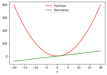
In the two plot() function above, we extract the values from PyTorch tensors so we can visualize them. The .detach method doesn’t allow the graph to further track the operations. This makes it easy for us to convert a tensor to a numpy array.

Summary

In this tutorial, you learned how to implement derivatives on various functions in PyTorch.

Particularly, you learned:

• How to calculate derivatives in PyTorch.
• How to use autograd in PyTorch to perform auto differentiation on tensors.
• About the computation graph that involves different nodes and leaves, allowing you to calculate the gradients in a simple possible manner (using the chain rule).
• How to calculate partial derivatives in PyTorch.
• How to implement the derivative of functions with respect to multiple values.

Tweet Tweet Share Share

The post Calculating Derivatives in PyTorch appeared first on Machine Learning Mastery.

source https://machinelearningmastery.com/calculating-derivatives-in-pytorch/

The brain’s secret to life-long learning can now come as hardware for artificial intelligence

As companies use more and more data to improve how AI recognizes images, learns languages and carries out other complex tasks, a recent article shows a way that computer chips could dynamically rewire themselves to take in new data like the brain does, helping AI to keep learning over time.

source https://www.sciencedaily.com/releases/2022/02/220203160544.htm

People prefer interacting with female robots in hotels, study finds

People are more comfortable talking to female rather than male robots working in service roles in hotels, according to new research. The study, which surveyed about 170 people on hypothetical service robot scenarios, also found that the preference was stronger when the robots were described as having more human features.

source https://www.sciencedaily.com/releases/2022/02/220203083556.htm

Scientists develop insect-sized flying robots with flapping wings

A new drive system for flapping wing autonomous robots has been developed, using a new method of electromechanical zipping that does away with the need for conventional motors and gears.

source https://www.sciencedaily.com/releases/2022/02/220202143053.htm